Product Resale Price Prediction using Machine Learning — a Case Study

Price-prediction using Regression.

Introduction

It’s safe to say that artificial intelligence (AI) is changing every aspect of modern living. From our smartphones to healthcare to security and every other industry, AI is slowly but surely becoming a common part of today’s environment, deeply embedded in everything we do. Retail is no exception, entering a new era of predictive commerce.

In this post, we’ll focus on how one can leverage Machine Learning techniques to help with a tricky aspect of retail — pricing.

Business Problem

Image source : clickmeeting

In recent years, the ecommerce market has grown significantly and continues to grow at a very steady pace in most countries. People are finding it more convenient to sit at home and order products ranging from electronics to groceries .

The E-commerce market in India is also set to grow at a CAGR of 30% for gross merchandise value to reach 200 bn dollars by 2026, and have a market penetration of 12% compared to 2% currently. This growth in online marketplaces has also invoked interest in building machine learning systems that help in predicting product prices of both new and used products , forecasting sales,etc. Accurate price prediction could provide companies an upper hand over competitors in terms of sales & ROI.

But, it can be hard to know how much something’s really worth. Small details can mean big differences in pricing. For example, one of these sweaters cost 335 dollars and the other cost 9.99 dollars. Can you guess which one’s which?

Image source : kaggle

Product pricing gets even harder at scale, considering just how many products are sold online. Clothing has strong seasonal pricing trends and is heavily influenced by brand names, while electronics have fluctuating prices based on product specs.

Mercari , Japan’s biggest community-powered shopping app, knows this problem deeply. They’d like to offer pricing suggestions to sellers, but this is tough especially because their sellers are enabled to put just about anything, or any bundle of things, on Mercari’s marketplace.

Problem Statement :

Build an algorithm that automatically suggests the right product resale prices.

Source — https://www.kaggle.com/c/mercari-price-suggestion-challenge/overview

Real World / Business Objectives and Constraints :

1. Predict product prices as accurately as possible.
2. Incorrect price tags could hamper customer experience and effect product sales negatively. ↓

1. Data Information

Source :

It is a 3-yr old Kaggle problem.

Link — https://www.kaggle.com/c/mercari-price-suggestion-challenge/overview

Overview :

• Train.tsv contains 8 columns : train_id, name, item_condition_id,category_name, brand_name, price,shipping,item_description
• Test.tsv contains all the same columns but the “price” column which is to be predicted
• Size of Train.tsv : 1482 K
• Size of Test.tsv : 34607 K

Data Fields :

Independent variables :-

1. train_id or test_id — the id of the listing
2. name — the title of the listing. Data has been cleaned to remove text that look like prices (e.g. $20) to avoid leakage. These removed prices are represented as [rm]
3. item_condition_id — the condition of the items provided by the seller
4. category_name — category of the listing
5. shipping — 1 if shipping fee is paid by seller and 0 by buyer
6. item_description — the full description of the item. Data has been cleaned to remove text that look like prices to avoid leakage. These removed prices are represented as [rm]

Dependent variable :-

1. price — the price that the item was sold for. This is the target variable that has top be predicted. The unit is USD. This column doesn’t exist in test.tsv

2. ML Problem Formulation

Image source : SGAnalytics

The data has 6 independent variables with a mix of text, categorical & numerical variables, and one continuous dependant variable. It looks like a standard regression problem.

Performance/Evaluation metric :

The evaluation metric for this problem is Root Mean Squared Logarithmic Error (RMLSE).

RMSLE is calculated as :

Where:

• ϵ is the RMSLE value (score)
• n is the total number of observations in the (public/private) data set,
• pi is your prediction of price, and
• ai is the actual sale price for i.
• log(x) is the natural logarithm of x.

RMLSE is the preferred evaluation metric since :

• It is a more robust measurement of error in comparison to other metrics like RMSE and R-square. In case of RMSE or R-square, the presence of outliers would cause the error value to explode. But RMLSE scales down the errors to a great extent.
• RMLSE, internally, captures the relative error between the predicted and the actual values. Since , due to the property of log, we can derive this : (log(pi + 1) — log(ai + 1)) = log( log(pi + 1)/log(ai + 1) ) .
• Thus, only the relative error matters, not the scale of error.
• RMLSE incurs a larger penalty for the underestimation of the actual variable than the overestimation. Maybe this is helpful here since the sellers would incur losses if the estimated/predicted selling price is lower than the actual selling price of the product.

3. Existing Approaches and My Approaches

Existing Approaches :

1. Strategic Pricing of Used Products for e-Commerce Sites :BOW technique is used to vectorize the “product name” since it is a small text feature & TFIDF is used to vectorize “product description, and the categorical features are vectorized using LabelBinarizer. ML techniques like Ridge Regression & LightGBM on the final dataset.
2. Mercari Golf : An ensemble of 4 MLP models, each model having the same architecture but being trained on 2 different datasets.

My Approaches :

ML Techniques :

Linear Regression, Ridge Regression, SVR Regression and Light GBM Regression.

DL Techniques :

The existing DL approaches have built complex ensembles to achieve lower error. I’ve tried to build a single model that would also predict the prices accurately and reduce the error(RMLSE). I’ve tried three model architechtures :

• 1DConv+LSTM on Text features and Dense Network on the other features.
• Dense Network on BOW vectorized features.
• Dense Network on TFIDF vectorized features.

4. EDA

Exploratory Data Analysis refers to the critical process of performing initial investigations on data so as to discover patterns, to spot anomalies, to test hypothesis and to check assumptions with the help of summary statistics and graphical representations.

On first glance, the data looks like this :

Observations :

• We don’t require the “train_id” column for our task. So, we’ll remove it.
• There are some missing (NaN) values in “brand_name” column. We’ll investigate missing values in a while.
• There are some data points where “item_description” has not been provided, denoted by — “No description yet”.
• Column ‘category_name’ has sub divisions, thus we split it into main category and sub categories.

4.1 Checking for missing values :

Lets plot the missing value statistics using “missingno” library :

• Feature ‘brand_name’ has a lot of missing values. So, we’ll try and impute them in a while.
• ‘category_name’ & ‘item_description’ also have missing values but their count is very less. So, we’ll just replace the missing values by “missing”

4.2 Splitting “category_name ” :

4.3 Univariate Analysis :

Price :

• Median price is 17$ whereas the highest price is 2009$ . From the percentiles, we can see that there is a big gap between 90th & 100th percentile price.
• Some products also have price = 0$. So, we’ll have to remove those data points.

• On further investigation, we find that the 99th percentile is still far off from the highest price, so we can expect a very few number of products to have abnormally large prices .

Item Condition :

• Maximum number of items are of category 1 and the least number of items belongs to category 5. We can assume that item-condition1 refers to the items that are in the best condition since the products that are in the best condition should be more sellable.

• The median price seems to decrease slightly from item condtion 1–4.
• Median price of item condtion 5 is slightly higher but number of points in this category is very less so we can say there is a decreasing trend in prices as we go from item condition 1 to 4.

Shipping :

• There are more number of products whose shipping has been paid by the buyer as compared to those whose shipping has been paid by the seller.

• Items whose shipping price is paid by buyers have higher median price. Thus ‘shipping’ can be an useful feature for our model.
• This might be as data points where shipping price is paid by customers/buyers are more sellable due to whichever reason such that customers are willing to pay more even after bearing the cost of shipping themselves.

Main Category :

• Most products sold are of category- Women and Beauty, maybe because women are likely to shop more and maybe they buy more Beauty products.

• Median prices for Men & Women category products are higher than other categories.
• Median prices of the other categories are sligtly lower but are in close range.
• Thus, main_cat could be an useful category for predicting between the price.

Sub Category-1 :

• Athletic Apparel, Makeup , Tops&Blouses and Shoes are the top 4 most popular product subcategories, followed by Jewellery,Toys, Cell Phones & Accessories, etc .

• There is a huge variance in median prices across the different subcategory-1 groups. Products of some categories have much higher median prices than some others.
• So , this feature will certainly be useful in predicting the product price.

Sub Category-2 :

• Pants,Tights,Leggings is the most popular sub-category(2) followed by Face, Tshirts,etc.
• We can assume that Pants , Tights or Leggings would fall under ‘Sports’ sub-category(1) and Face could fall under ‘Makeup’ sub-category(1), thus having higher counts.

• There is also a considerable variance in median prices across the different subcategory-2 groups.
• So , this feature will also be useful in predicting the product price.

Brand Name :

As we saw earlier, brand Names are missing in some data points, we’ll try to impute the values in a while.

For now, lets analyse the given data, apart from the data points where “brand_name” is missing :

• Most popular brand names are :

1. PINK(Women’s clothing)

2. NIKE(Sports)

3. Victoria’s Secret(Women’s)

4. LulaRoe(Fashion)

Checking Median prices fetched by brands :

• Most brands fetch prices below 200$. However, there are a few exceptions.

Lets investigate those brands :

• Some brands like David Yurman, Vitamix,Blendtec have very high median prices but their frequency is very less compared to the size of the data set. So, their importance might not be that significant.

4.4 Imputing “brand_name” values :

Brand Names are missing in 42% of data points.

• In our analysis, we found that we can find the “brand_name” values from “item_description” and “name” columns also. Thus, we’ll try to impute the missing brand names from these 2 columns.
• Here, the amount of data is huge, so we have to leverage multiprocessing for our task of finding & imputing brand names :

Let’s check the results of imputation :

• We could successfully impute close to half of the missing values. So, we’ll replace all the remaining ‘NaN’ values in the dataset by “missing” and drop the original “brand_name” column.

4.5 Multivariate Analysis :

Let’s bin our data into 3 groups, so that it helps us in analysis :

• price < 14$ : Cheap
• 14$ ≤ price ≤ 26$ : Affordable
• price > 26$ : Expensive

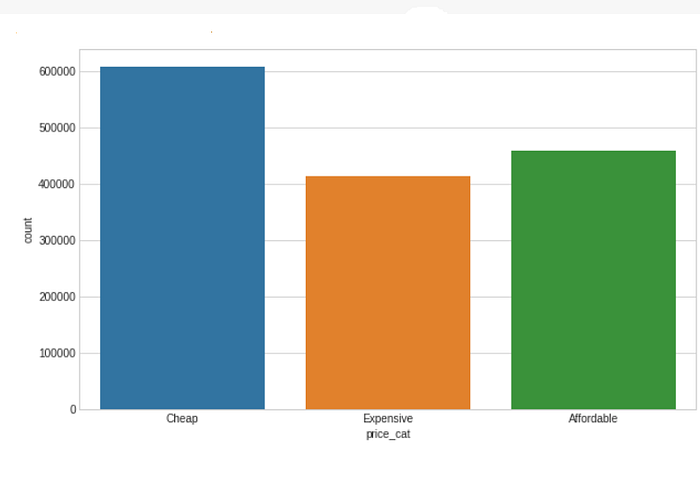
• Most number of products are Cheap, followed by Affordable and Expensive products.

Let’s check top 10 most sold brands and what prices their products fetch :

• Most brands have products of different price categories except brands like ‘Michael Kors’ and ‘Lululemon’ where most products are Expensive.

Now, let’s check how the prices of these brands vary with the item condition of the products sold :

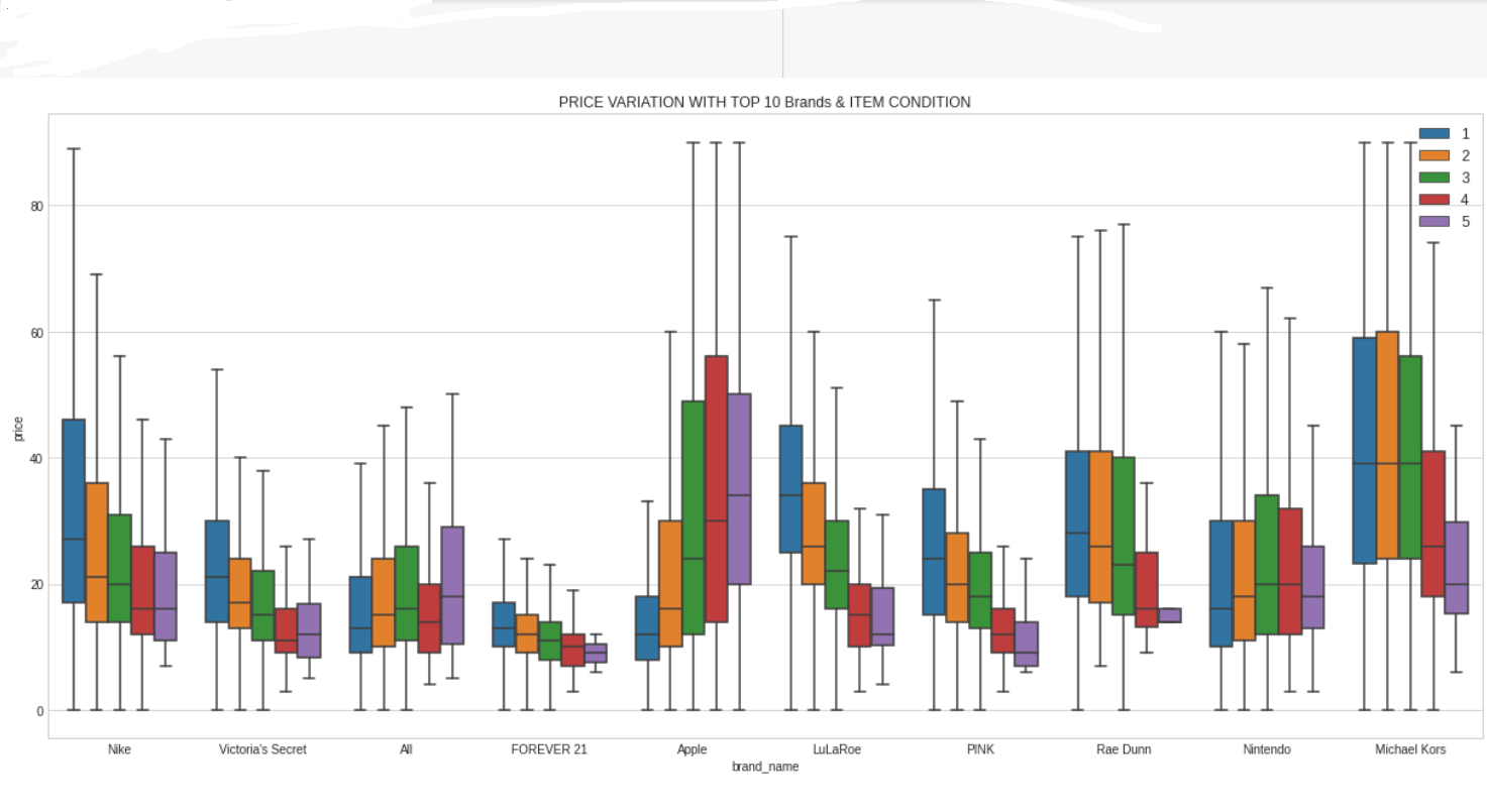
• The combination of attributes ‘item_condition_id’ & ‘brand_name’ of top 10 brands can differentiate the product prices to a good extent.

4.6 Summary of Observations :

‘item_condition_id’ — Prices decrease slightly as the item condition worsens. But, this attribute in combination with ‘main_cat’ (i.e the main category of products) produces a variation in product prices.

‘shipping’ — Across products of almost all brands & categories, products for which the buyer paid shipping charges have higher prices than for those which the seller paid shipping.

‘brand_name’ — Median product prices vary across brands. The brand name in combnation with other attributes like item_condition_id and main_cat produce interesting variation of product prices.

‘main_cat’ — Product Median Prices vary across different Main Category types. main_cat along with other features produce variations in product price. So, it’s an important feature.

‘sub_cat1’ — Product Median Prices vary across different Sub Category-1 types.

‘sub_cat2’ — Product Median Prices vary across different Sub Category-2 types.

5. Data Cleaning and Preprocessing :

5.1 Categorical Features :

As we can see, there are some non-alphanumeric characters in the all the 3 categories — main_cat,sub_Cat1 and sub_cat2.

Thus, we clean the 3 category columns :

5.2 Text Features :

“item_description” —

It’s a routine task to preprocess the text features. We clean and preprocess the “item_description” values.

“name” —

6. Feature Engineering Attempts :

Tried to engineer some new features but didn’t find them to be quite useful :

• None of the features have a stong enough correlation with the target variable. So, we discard them .

7. Preparing Train and Test Data :

Intial Train-Test Split :

Removed the unwanted columns and split the training data provided from Kaggle into Train & Test Datasets

The data looks like this :

We’ll prepare three Datasets to experiment —

• Bag Of Words(BOW) featurized data
• TF-IDF featurized data
• Tokenized text & Sparse data

7.1 Bag Of Words(BOW) featurized data :

We will use CountVectorizer to BOW vectorize our Text and Categorical features. Lets us first understand how CountVectorizer works :

Scikit-learn’s CountVectorizer is used to convert a collection of text documents to a vector of term/token counts. It also enables the ​pre-processing of text data prior to generating the vector representation. This functionality makes it a highly flexible feature representation module for text.

Image source : Geeksforgeeks

Text Features :

BOW featurized text features using sklearn’s CountVectorizer-

Categorical Features :

BOW featurized categorical features using sklearn’s CountVectorizer-

Numerical Features :

We use sklearn’s MinMaxScaler for scaler our numerical features .

MinMaxScaler scales all the data features in the range [0, 1] (by default) or else in the range [-1, 1] if there are negative values in the dataset .

Image Source : Geeksforgeeks

We use MinMaxScaler to scale “item_condition_id” :

Target Variable :

We also have to convert target variable to logarithmic scale so that we can use root mean square error as the metric instead of explicitly defining RMLSE.

We will use Numpy’s log1p() function for this :

Preparing final dataset :

We use Scipy’s hstack() function to stack our vectorized features and create the final dataset that will be used for training :

7.2 TF-IDF featurized data :

TF-IDF stands for Term Frequency — Inverse Document Frequency.

TF-IDF is a score which is applied to every word in every document in our dataset. And for every word, the TF-IDF value increases with every appearance of the word in a document, but is gradually decreased with every appearance in other documents.

• In simplest terms, we can say that TF-IDF value would be high for those rare words that occur multiple times only in very few documents but are seldom present in other documents.
• Similarly, TF-IDF value would be lower if the specific word occurs in many documents and isn’t a rarity.

It’s a concept that is difficult to explain in few lines. If you want to know more , you can check this link.

Text Features :

We vectorize the ‘item_description’ feature using Sklearn’s TfidfVectorizer :

Preparing final dataset :

We use the Tf-idf vectorized “item_description” data and the rest from the BOW features :

7.3 Tokenized text & Sparse data :

We’ll vectorize the text feature ‘item_description’ using Tokenizer and pad_sequences() :

tf.keras.preprocessing.text.Tokenizer : This class allows to vectorize a text corpus, by turning each text into either a sequence of integers (each integer being the index of a token in a dictionary)

tf.keras.preprocessing.sequence.pad_sequences : Pads sequences to the same length.

Since every document may have different number of total words, their tokenized sequences will also be of different lengths. Thus, we need to pad the tokenized sequences so that they are of the same length.

Vectorizing ‘item_description’ and ‘name :

Non-text Features :

Preparing final dataset :

We’ll get the final dataset for training by combining the encoded text features and the non-text features :

Train = [padded_description_train, padded_name_train, X_tr_nontxt]

Test = [padded_description_test, padded_name_test, X_te_nontxt]

8. Training & Testing ML/DL Models:

8.1 ML Models :

Let’s train the following regression models and evaluate their performance on Test data :

• Linear Regression (Baseline) — Linear Least Square
• Ridge Regression — Linear Least Square with L2 Regularization
• SVR Regression — Epsilon-Insensitive Loss(Soft- margin SVM)
• Light-GBM Regression — Light Gradient Boosting Machine

Linear Regression :

Linear regression attempts to model the relationship between two variables by fitting a linear equation to observed data. One variable is considered to be an explanatory variable, and the other is considered to be a dependent variable.

We’ll keep this model as our baseline. Let’s fit the data and test the model :

RMLSE on TRAIN Data = 0.44788603982109476

RMLSE on TEST Data = 0.46807207137757767

Kaggle RMLSE = 0.47660

Ridge Regression :

This model solves a regression model where the loss function is the linear least squares function and regularization is given by the l2-norm. We can modify the value of ‘alpha’ i.e the regularization strength and choose the best value for our data.

We’ll do hyperparameter-tuning and then train the final model with the best parameters.

RMLSE on TRAIN Data = 0.44196214665140854

RMLSE on TEST Data = 0.4609332745825652

Kaggle RMLSE = 0.46853

SVR Regression :

In simple regression we try to minimise the error rate. While in SVR we try to keep the error within a certain threshold.

We’ll do hyperparameter-tuning and then train the final model with the best parameters :

RMLSE on TRAIN Data = 0.47556175648468174

RMLSE on TEST Data = 0.4809737240617147

Kaggle RMLSE = 0.48818

Light-GBM Regression :

Light GBM is a fast, distributed, high-performance gradient boosting framework based on decision tree algorithm, used for ranking, classification and many other machine learning tasks.

Since it is based on decision tree algorithms, it splits the tree leaf wise with the best fit whereas other boosting algorithms split the tree depth wise or level wise rather than leaf-wise. So when growing on the same leaf in Light GBM, the leaf-wise algorithm can reduce more loss than the level-wise algorithm and hence results in much better accuracy which can rarely be achieved by any of the existing boosting algorithms. Also, it is very fast, hence the word ‘Light’.

RMLSE on TRAIN Data = 0.4164715508973795

RMLSE on TEST Data = 0.45097900374349953

Kaggle RMLSE = 0.45830

8.2 DL Models :

Done with the ML models. Now, let’s check how the Deep Learning techniques perform on the data.

1DConv+LSTM on Text features and Dense Network on the other features :

Conv+LSTMs can be useful for text features. Recurrent neural networks can obtain context information from text and Convolutional neural network (CNN) can obtain important features of text through pooling. Let’s try out this model structure and see how it performs.

Model Architecture —

Let’s fit the model to data and test it’s performance :

RMLSE on TRAIN Data = 0.40325830205299756

RMLSE on TEST Data = 0.4522887404428894

Kaggle RMLSE = 0.46145

Dense Network on BOW vectorized features :

Model Artitecture :

Let’s fit the model to data and test it’s performance :

RMLSE on TRAIN Data = 0.37576717294003453

RMLSE on TEST Data = 0.43891317200216107

Kaggle RMLSE = 0.44675

Dense Network on TFIDF vectorized features :

Model Artitecture :

Let’s fit the model to data and test it’s performance :

RMLSE on TRAIN Data = 0.4124439548671445

RMLSE on TEST Data = 0.4440186551467468

Kaggle RMLSE = 0.45247

Comparison of Models :

Let’s analyse how all the models performed in comparison to each other :

Dense Network with BOW features performs the best. We’ll choose this model to be our final model.

Future Work :

• One can always try complex ensembles. They would produce better results but affect latency of the model.
• We can try out more complex Deep Learning architechtures but be wary of the models overfitting to Train data.
• We can try different vectorization parameters.
• We can try different kinds of DL units like GRUs, Bidirectional LSTMs, etc.

Conclusion :

It was an engaging task.There’s a mixture of all kinds of features and a lot of data preprocessing was required. I’ve tried to experiment with a few techniques that haven’t been tried on this data before.

For full — length code, you can check out the github link.

For any suggestions/questions , you can connect with me on linkedin.

References :

1. Strategic Pricing of Used Products for e-Commerce Sites (iastate.edu)
2. Machine Learning for Retail Price Recommendation with Python | by Susan Li | Towards Data Science
3. https://medium.com/@mrunal68/text-sentiments-classification-with-cnn-and-lstm-f92652bc29fd
4. https://machinelearningmastery.com/prepare-text-data-deep-learning-keras/
5. https://www.appliedaicourse.com/course/11/Applied-Machine-learning-course